
The foundational histogramming package for Python, boost-histogram, hit beta status with version 0.6! This is a major update to the new Boost.Histogram bindings. Since I have not written about boost-histogram yet here, I will introduce the library in its current state. Version 0.6.2 was based on the recently released Boost C++ Libraries 1.72 Histogram package. Feel free to visit the docs, or keep reading this post.
This Python library is part of a larger picture in the Scikit-HEP ecosystem of tools for Particle Physics and is funded by DIANA/HEP and IRIS-HEP. It is the core library for making and manipulating histograms. Other packages are under development to provide a complete set of tools to work with and visualize histograms. The Aghast package is designed to convert between popular histogram formats, and the Hist package will be designed to make common analysis tasks simple, like plotting via tools such as the mplhep package. Hist and Aghast will be initially driven by HEP (High Energy Physics and Particle Physics) needs, but outside issues and contributions are welcome and encouraged.
The key design feature of the boost-histogram package (and the C++ library on which it is based) is the idea of a configurable and highly performant Histogram object. A histogram is made of two things: a storage and a collection of axes.
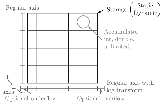
There are a preset collection of storages in boost-histogram, with different
datatypes. Storages can hold simple data types (Int64, Double, and
AtomicInt64), a special mutating Unlimited datatype that starts as an 8 bit
int and grows, and even converts to double if weights are used (or, currently,
if a view is requested). There are also several accumulators. You can use
WeightedSum to track an error1, or Mean / WeightedMean to implement a
“profile” histogram.
Axes come in a variety of flavors. Regular provides even bin spacings,
Variable provides arbitrary bin spacings, Integer is a high performance
simple integer spacing, and IntCategory / StrCategory provide arbitrary
non-continuous categories. Each of these has options, such as growth=, which
allows the axis to grow when out-of-range fills are made, overflow= and
underflow=, which hold out-of-range fills on continuous axes, and circular=,
which causes an axis to wrap around. The Regular axis also supports
transforms, which map values in and out of the regular binning space. A
few common transforms are provided, such as Pow(v), sqrt, and log, and
users can supply a pair of CTypes function pointers to build new transforms with
full performance. Feel free to use numba.cfunc to write your transforms
directly in Python!
Usage example
Let’s take a look at what using the library looks like. Let’s start with a simple, contrived 1D dataset:
import numpy as np
import boost_histogram as bh
import matplotlib.pyplot as plt

norm_vals = np.concatenate(
    [
        np.random.normal(loc=5, scale=1, size=1_000_000),
        np.random.normal(loc=2, scale=0.2, size=200_000),
        np.random.normal(loc=8, scale=0.2, size=200_000),
    ]
)
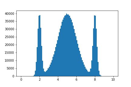
This has a large Gaussian peak at 5, with two narrow peaks at 2 and 8. Using the boost-histogram API, we would make a histogram object with a regular binning. We want 100 bins from 0 to 10:
hist = bh.Histogram(
    bh.axis.Regular(100, 0, 10),
)
Now, we can call .fill to fill the histogram in-place:
hist.fill(norm_vals)
Histogram(Regular(100, 0, 10), storage=Double()) # Sum: 1399999.0 (1400000.0 with flow)
The histogram has a nice representation on the command line that includes the
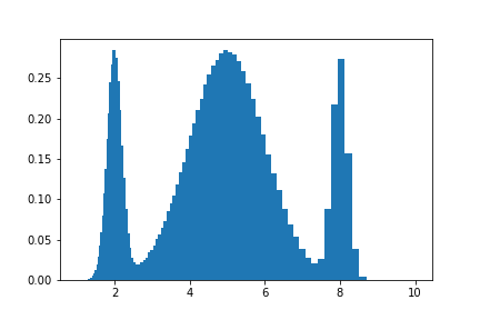
sum (both with and without the extra flow bins). If we want to plot densities,
boost-histogram does not currently have a .density method/property, but you
can easily use the built-in properties to compute it:
# Compute the "volume" of each bin (useful for 2D+)
volumes = np.prod(hist.axes.widths, axis=0)

# Compute the density of each bin
density = hist.view() / hist.sum() / volumes
The above code works on any number of dimensions, not just 1D histograms!
Now, plotting is also simple, using the same collection of properties:
plt.bar(*hist.axes.centers, density, *hist.axes.widths)
Since axes returns a tuple of items, we use * to unpack the only item
(axes[0]), but you can just directly call axes[0] if you prefer.
We could use any other axis, or a transformed axis, and the downstream code would not change:
hist = bh.Histogram(
    bh.axis.Regular(100, 1, 10, transform=bh.axis.transform.log),
)

hist.fill(norm_vals)

volumes = np.prod(hist.axes.widths, axis=0)
density = hist.view() / hist.sum() / volumes

plt.bar(*hist.axes.centers, density, *hist.axes.widths)
NumPy comparison
If you are familiar with NumPy, the equivalent code for the simple regular binning in NumPy would be:
%%timeit
bins, edges = np.histogram(norm_vals, bins=100, range=(0, 10))
17.4 ms ± 2.64 ms per loop (mean ± std. dev. of 7 runs, 100 loops each)
Of course, you then are either left on your own to compute centers, density,
widths, and more, or in some cases you can change the computation call itself to
add density=, or use the matching function inside Matplotlib, and the API is
different if you want 2D or ND histograms. But if you already use NumPy
histograms and you really don’t want to rewrite your code, boost-histogram has
adaptors for the three histogram functions in NumPy:
%%timeit
bins, edges = bh.numpy.histogram(norm_vals, bins=100, range=(0, 10))
7.3 ms ± 55.7 µs per loop (mean ± std. dev. of 7 runs, 100 loops each)
This is only a hair slower2 than using the raw boost-histogram API, and is still a nice performance boost over NumPy. You can even use the NumPy syntax if you want a boost-histogram object later:
hist = bh.numpy.histogram(norm_vals, bins=100, range=(0, 10), histogram=bh.Histogram)
You can later get a NumPy style output tuple from a histogram object:
bins, edges = hist.to_numpy()
So you can transition your code slowly to boost-histogram.
ND histograms
All the above concepts (except for plotting details) expand gracefully to
multiple dimensions. The .axes object can be indexed as a tuple, or it can
directly call any method or property of the axes and return the results as a
tuple. If the result is an array, the returned iterable of arrays will be ready
for broadcasting, as well; this is why the above density calculation works
regardless of the number of axes in your histogram.
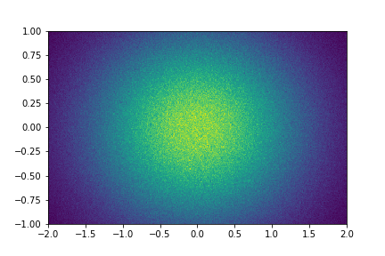
h2 = bh.Histogram(bh.axis.Regular(400, -2, 2), bh.axis.Regular(200, -1, 1))

data = np.random.multivariate_normal((0, 0), ((1, 0), (0, 0.5)), 10_000_000).T.copy()

h2.fill(*data)

# pcolormesh requires xy indexing, we produce ij for consistency with higher dimensions
x, y = h2.axes.edges
plt.pcolormesh(x.T, y.T, h2.view().T)

# Or you could do:
edges = h2.axes.edges
plt.pcolormesh(*np.broadcast_arrays(h2.axes.edges), h2)
Histograms support the NumPy array protocol, so can often be used directly in places like plotting code instead of calling
.view().
We can check the performance against NumPy again; NumPy does not do well with regular spaced bins in more than 1D:
%%timeit
np.histogram2d(*data, bins=(400, 200), range=((-2,2), (-1, 1)))
1.31 s ± 17.3 ms per loop (mean ± std. dev. of 7 runs, 1 loop each)
%%timeit
bh.numpy.histogram2d(*data, bins=(400, 200), range=((-2,2), (-1, 1)))
101 ms ± 117 µs per loop (mean ± std. dev. of 7 runs, 10 loops each)
For more than one dimension, boost-histogram is more than an order of magnitude faster than NumPy for regular spaced binning. Although optimizations may be added to boost-histogram for common axes combinations later, in 0.6.2, all axes combinations share a common code base, so you can expect at least this level of performance regardless of the axes types or number of axes!
Unified Histogram Indexing (UHI)
One of the key developments in boost-histogram is the indexing system, known
as UHI. It was designed so that the indexing “tags” could be shared across
libraries, and (in some cases) be implemented by users. The design of UHI
follows NumPy indexing when NumPy is valid, that is, h[foo] == h.view()[foo]
for all foo that is valid for both histograms and arrays. Any other valid
foo for one should be invalid for the other. For example, histograms do not
support integer steps. NumPy arrays do not support the callables listed below.
For a histogram, the slice should be thought of like this:
histogram[start:stop:action]
The start and stop can be either a bin number (following Python rules), or a
callable; the callable will get the axis being acted on and should return an
extended bin number (-1 and len(ax) are flow bins). A provided callable is
bh.loc, which converts from axis data coordinates into bin number.
The final argument, action, is special. A general API is being worked on, but
for now, bh.sum will “project out” or “integrate over” an axes, and
bh.rebin(n) will rebin by an integral factor. Both work correctly with limits;
bh.sum will remove flow bins if given a range. h[0:len:bh.sum] will sum
without the flow bins.
Here are a few examples that highlight the functionality of UHI:
Example 1
You want to slice axis 0 from 0 to 20, axis 1 from .5 to 1.5 in data coordinates, axis 2 needs to have double size bins (rebin by 2), and axis 3 should be summed over. You have a 4D histogram.
Solution:
ans = h[:20, bh.loc(-0.5) : bh.loc(1.5), :: bh.rebin(2), :: bh.sum]
Example 2
You want to set all bins above 4.0 in data coordinates to 0 on a 1D histogram.
Solution:
h[bh.loc(4.0) :] = 0
You can set with an array, as well. The array can either be the same length as the range you give, or the same length as the range + under/overflows if the range is open ended (no limit given). For example:
h = bh.Histogram(bh.axis.Regular(10, 0, 1))
h[:] = np.ones(10)  # underflow/overflow still 0
h[:] = np.ones(12)  # underflow/overflow now set too
Note that for clarity, while basic NumPy broadcasting is supported, axis-adding broadcasting is not supported; you must set a 2D histogram with a 2D array or a scalar, not a 1D array.
Example 3
You want to sum from -infinity to 2.4 in data coordinates in axis 1, leaving all other axes alone. You have an ND histogram, with N >= 2.
Solution:
ans = h[:, : bh.loc(2.4) : bh.sum, ...]
Notice that last example could be hard to write if the axis number, 1 in this
case, was large or programmatically defined. In these cases, you can pass a
dictionary of {axis:slice} into the indexing operation. A shortcut to quickly
generate slices is provided, as well:
ans = h[{1: slice(None, bh.loc(2.4), bh.sum)}]

# Identical:
s = bh.tag.Slicer()
ans = h[{1: s[: bh.loc(2.4) : bh.sum]}]
Example 4
You want the underflow bin of a 1D histogram.
Solution:
val = h1[bh.underflow]
Analyses using axes
Taken together, the flexibility in axes and the tools to easily sum over axes can be applied to transform the way you approach analysis with histograms. For example, let’s say you are presented with the following data in a 3xN table:
| Data | Details |
|---|---|
value | |
is_valid | True or False |
run_number | A collection of integers |
In a traditional analysis, you might bin over value where is_valid is True,
and then make a collection of histograms, one for each run number. With
boost-histogram, you can make a single histogram, and use an axis for each:
value_ax = bh.axis.Regular(100, -5, 5)
bool_ax = bh.axis.Integer(0, 2, underflow=False, overflow=False)
run_number_ax = bh.axis.IntCategory([], growth=True)

hist = bh.Histogram(value_ax, bool_ax, run_number_ax)

hist.fill([-2, 2, 4, 3], [True, False, True, True], [3, 5, 5, 7])
Histogram(
  Regular(100, -5, 5),
  Integer(0, 2, underflow=False, overflow=False),
  IntCategory([3, 5, 7], growth=True),
  storage=Double()) # Sum: 4.0
Now, you can use these axes to create a single histogram that you can fill. If
you want to get a histogram of all run numbers and just the True is_valid
selection, you can use a sum:
hist[:, bh.loc(True), :: bh.sum]
Histogram(Regular(100, -5, 5), storage=Double()) # Sum: 3.0
If you want to pick a single category value, just use bh.loc(item). A range or
set of values cannot be selected, but you can use a generator expression:
from functools import reduce
from operator import add

reduce(add, (hist[:, bh.loc(True), bh.loc(item)] for item in {3, 5}))
Histogram(Regular(100, -5, 5), storage=Double()) # Sum: 2.0
You should note that in the above examples, the index and the bin are the same for boolean axes (or any integer axis that starts at 0). So you can use
Truedirectly instead ofbh.loc(True)if you prefer.
You can expand this example to any number of dimensions, boolean flags, and categories.
Accumulator storages
There are three accumulator-based storages. WeightedSum keeps track of both a
weighted sum (like Double) and also a variance. Profile histograms track a
Mean (or a WeightedMean) instead of a sum; this is available as well. These
types return accumulators when asked for a single value, or a NumPy record
array-like view when asked for a view. This is done without copying the data,
and you can also access a few computed properties. Here’s an example:
hm = bh.Histogram(
    bh.axis.Regular(20, -1.5, 1.5, underflow=False, overflow=False),
    storage=bh.storage.Mean(),
)

# Interesting data
data = np.random.multivariate_normal(
    (0, 1), ((0.1, 0.3), (0.3, 1.0)), size=10_000
).T.copy()

# Fill with sample
hm.fill(data[0], sample=data[1])

# Plot
fig, ax = plt.subplots()
ax.hist2d(*data, bins=100, cmap="gray_r")
ax.errorbar(
    hm.axes[0].centers, hm.view().value, yerr=np.sqrt(hm.view().variance), fmt="ro"
)
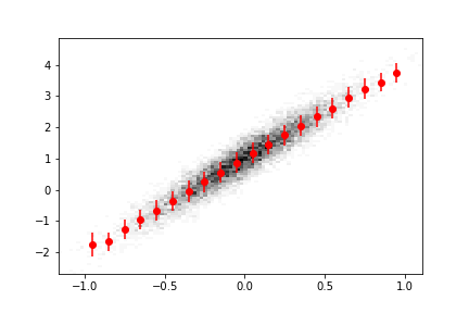
Here we have overlaid a Matplotlib 2D histogram with a boost-histogram 1D profile histogram.
The little details
The library respects Python conventions and interacts well with IPython wherever possible. Python 2 is still supported for the 1.0 release so that Python 2 users will be able to access histogramming, but care was taken to ensure Python 3 users do not suffer for this. For example, if you inspect a function signature, you will see the proper Python 3 signature if you are in Python 3:
Python 3 + IPython
bh.axis.Regular?
Init signature:
bh.axis.Regular(
    bins,
    start,
    stop,
    *,
    metadata=None,
    underflow=True,
    overflow=True,
    growth=False,
    circular=False,
    transform=None,
)
Python 2 + IPython
bh.axis.Regular?
Init signature:
bh.axis.Regular(
    bins,
    start,
    stop,
    **kwargs,
)
This means tab completion in IPython for Python 3 will properly suggest the keyword completions as you write, etc.
The histogram object behaves nicely when adding two histograms, multiplying or dividing by a scalar (depending on the storage), comparing histograms, printing histograms (try it with 1D!), setting with an array/view, accessing as a view, copying or deep-copying, and with any other expected Python manipulations or behaviours that are applicable to histograms. Currently, mismatched axes types or storages cannot be added, though this restriction may be carefully relaxed slightly in the future.
The library supports pickle3, and special care was taken to make sure histograms provide excellent pickle performance even with accumulator storages.
import boost_histogram as bh
import pickle
from pathlib import Path

h = bh.Histogram(bh.axis.Regular(2, -1, 1))

h_saved = Path("h_saved.pkl")

# Now save the histogram
with h_saved.open("wb") as f:
    pickle.dump(h, f, protocol=-1)

# And load
with h_saved.open("rb") as f:
    h = pickle.load(f)
Threaded filling
You can use boost-histogram to do threaded filling, as well; the GIL is released
during the filling process. Version 0.7.0 has a threads= argument that can be
used in regular or numpy filling. If you want to implement it yourself, such as
in 0.6.2, you can. For example, using concurrent.futures, you can do:
from concurrent.futures import ThreadPoolExecutor


def threaded_fill(hist, threads, *data):
    def fun(*args):
        return hist.copy().reset().fill(*args)

    chunks_list = [np.array_split(d, threads) for d in data]

    with ThreadPoolExecutor(threads) as pool:
        results = pool.map(fun, *chunks_list)

    for h in results:
        hist += h
Then, a fill would look like this:
import os

threads = os.cpu_count()
threaded_fill(hist, threads, vals)
This can give you a 2-4x speedup over single-threaded filling, depending on the situation and the number of cores. The number of items in the fill must be large enough to offset the cost of making histogram copies and summing them afterwards.
Obtaining boost-histogram
While the only requirement to build boost-histogram is a C++14 compatible compiler, this still takes some time and is not always available. A wheel building system was set up for boost-histogram, and is now being used in other Scikit-HEP packages. Each release produces a large collection of wheels that pip will install in a couple of seconds on most systems.
| System | Arch | Python versions |
|---|---|---|
| ManyLinux1 (custom GCC 9.2) | 64 & 32-bit | 2.7, 3.5, 3.6, 3.7, 3.8 |
| ManyLinux2010 | 64-bit | 2.7, 3.5, 3.6, 3.7, 3.8 |
| macOS 10.9+ | 64-bit | 2.7, 3.6, 3.7, 3.8 |
| Windows | 64 & 32-bit | 2.7, 3.6, 3.7, 3.8 |
You simply install with:
pip install boost-histogram
and pip will give you the appropriate wheel in most cases, and will fall back on a source build if you are not covered in the above list. Linux distributions such as Alpine and ClearLinux are usually the only outliers, but those tend to have modern compilers.
We also support Conda through Conda-Forge:
conda install -c conda-forge boost-histogram
All Conda-Forge platforms are supported, including ARM and PowerPC. The one exception is Python 2.7 on Windows, which is not supported due to the C++14 requirements.
Acknowledgements
This library was developed by Henry Schreiner and Hans Dembinski, and is based on the Boost.Histogram library, developed by Hans Dembinski and first released as part of the Boost libraries in version 1.70.
Support for this work was provided by the National Science Foundation cooperative agreement OAC-1836650 (IRIS-HEP) and OAC-1450377 (DIANA/HEP). Any opinions, findings, conclusions or recommendations expressed in this material are those of the authors and do not necessarily reflect the views of the National Science Foundation.
In ROOT, this is a histogram with
.Sumw2()called before filling. ↩︎About a 5% penalty for the above example. If you use the
bins='auto'feature of NumPy histograms, boost-histogram will be slower, because it calls NumPy to study the data to compute the bin edges. You can still use it to produce a boost-histogram object, however, so it is still quite useful. ↩︎Any protocol except protocol 0. In Python 2, this is the default, though several higher levels are available, and protocol 0 has dismal performance. ↩︎